- Count based N-Gram Language Models
- Neural N-Gram Language Models
- Recurrent Neural Network Language Models
A language model assigns a probability to a sequence of words, given the observed training text, how probable is this new utterance?
Most language models employ the chain rule to decompose the joint probability into a sequence of conditional probabilities: \[ p(w_1, w_2, w_3, ..., w_N) = p(w_1)p(w_2|w_1)p(w_3|w_1,w_2)*...*p(w_N|w_1,..w_{N-1}) \] Evaluating a Language Model
A good model assigns real utterances \(w_1^N\) from a language a high probability. This can be measured with cross entropy: \[ H(w_1^N) = -\frac{1}{N}\log_2p(w_1^N) \] Intuition : Cross entropy is a measure of how many bits are needed to encode text with our model.
Data
Language modelling is a time series prediction problem in which we must be careful to train on the past and test on the future.
If the corpus is composed of articles, it is best to ensure the test data is drawn from a disjoint set of articles to the training data.
Count based N-Gram Language Models
Markov assumption
- only previous history matters
- limited memory: only last \(k - 1\) words are included in history(older words less relevant)
- \(k\)-th order Markov model
e.g. 2-gram language model: \[ p(w_1, w_2, ..., w_n) \approx p(w_1)p(w_2|w_1)p(w_3|w_2)...p(w_n|w_{n-1}) \] Estimating Probabilities
Maximum likelihood estimation for 3-grams: \[ p(w_3|w_1, w_2) = \frac{count(w_1,w_2,w_3)}{count(w_1,w_2)} \] In our training corpus we may never observe this trigrams:
- Oxford Pimm's eater
- Oxford Pimm's drinker
If both have count 0 our smoothing methods will assign the same probability to them.
A better solution is to interpolate with the bigram probability.
- Pimm's eater
- Pimm's drinker
A simple approach is linear interpolation: \[ p_l(w_n|w_{n-1}, w_{n-2}) = \lambda_3p(w_n|w_{n-1}, w_{n-2})+\lambda_2p(w_n|w_{n-1})+\lambda_1p(w_n) \] where \(\lambda_3 + \lambda_2 + \lambda_1 = 1\).
Summary
Good
- Count based n-gram models are exceptionally scalable and able to be trained on trillions of words of data
- fast constant time evaluation of probabilities at best time
- sophisticated smoothing techniques match the empirical distribution of language
Bad
- Large ngrams are sparse, so hard to capture long dependencies
- symbolic nature does not capture correlations between semantically similary word distributions, e.g. cat <-> dog.
- similarly morphological regularities, running <-> jumping, or gender.
Neural N-Gram Language Models
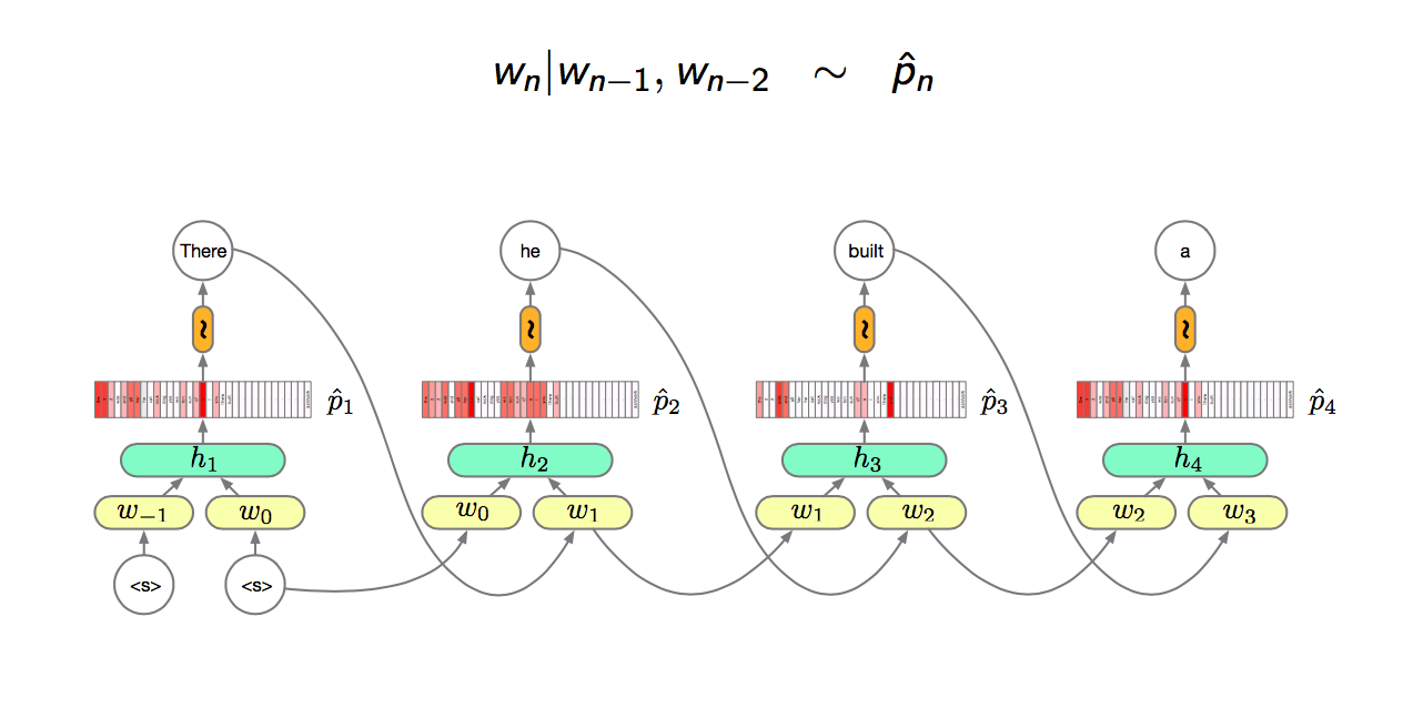
Trigram NN language model \[ h_n = g(V[w_{n-1};w_{n-2}] + c) \]
\[ \hat{p_n} = softmax(Wh_n + b) \]
\[ softmax(u)_i = \frac{\exp(u_i)}{\sum_j\exp u_j} \]
where
- \(w_i\) are one hot vetors and \(\hat{p_i}\) are distributions
- \(|w_i| = |\hat{p_i}| = V\) (words in the vocabulary)
- \(V\) is usually very large \(> 1e5\)
Training
The usual training objective is the cross entropy of the data given the model (MLE): \[
F = -\frac{1}{N}\sum_ncost_n(w_n,\hat{p_n})
\] The cost function is simply the model's estimated log-probability of \(w_n\): \[
cost(a, b) = a^T\log b
\] 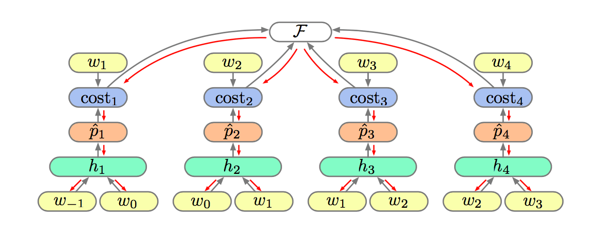
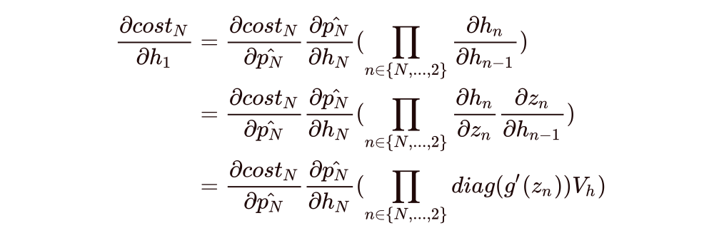
Calculating the gradients is straightforward with back propagation: \[ \frac{\partial F}{\partial W} = -\frac{1}{N}\sum_n \frac{\partial cost_n}{\partial \hat{p_n}}\frac{\partial \hat{p_n}}{\partial W} \]
\[ \frac{\partial F}{\partial W} = -\frac{1}{N} \sum_n\frac{\partial cost_n}{\partial \hat{p_n}}\frac{\partial\hat{p_n}}{\partial h_n}\frac{\partial h_n}{\partial V} \]
Comparison with Count Based N-Gram LMs
Good
Better generalisation on unseen n-grams, poorer on seen n-grams.
Solution: direct (linear) ngram features
Simple NLMs are often an order magnitude smaller in memory footprint than their vanilla n-gram cousins (though not if you use the linear features suggested above!)
Bad
- The number of parameters in the model scales with the n-gram size and thus the length of the history captured.
- The n-gram history is finite and thus there is limit on the longest dependencies that an be captured.
- Mostly trained with Maximum Likelihood based objectives which do not encode the expected frequencies of words a priori.
Recurrent Neural Network Language Models
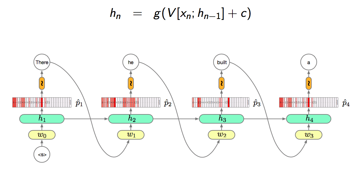
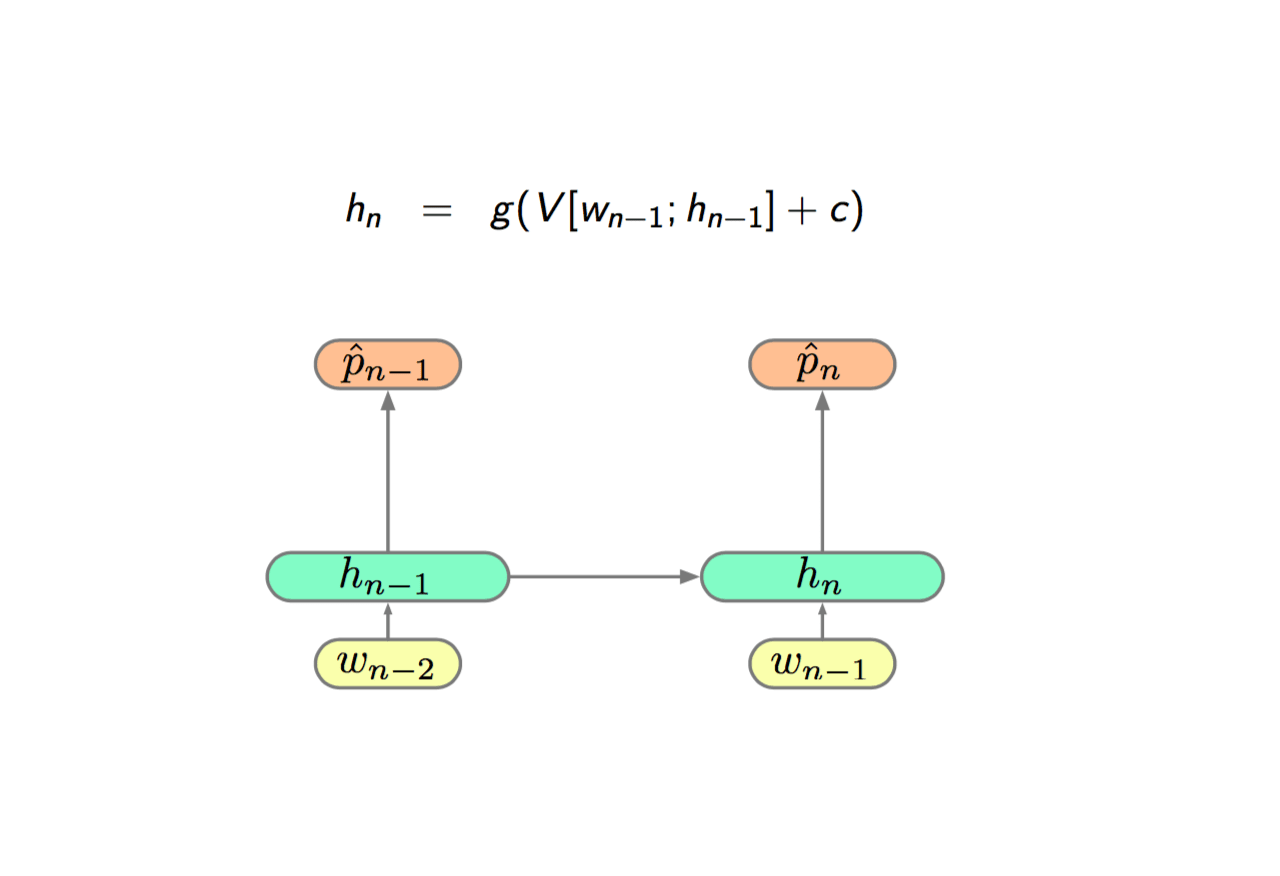
The major difference between RNN and Neural N-Gram model is RNN not only forward propagate the previous input (\(y_{n-1}\)) to next layer but also forward propagate the previous state (\(h_{n-1}\)).
BPTT
Back Propagation Through Time (BPTT) note the dependence of derivatives at time \(n\) with those at time \(n + \alpha\).
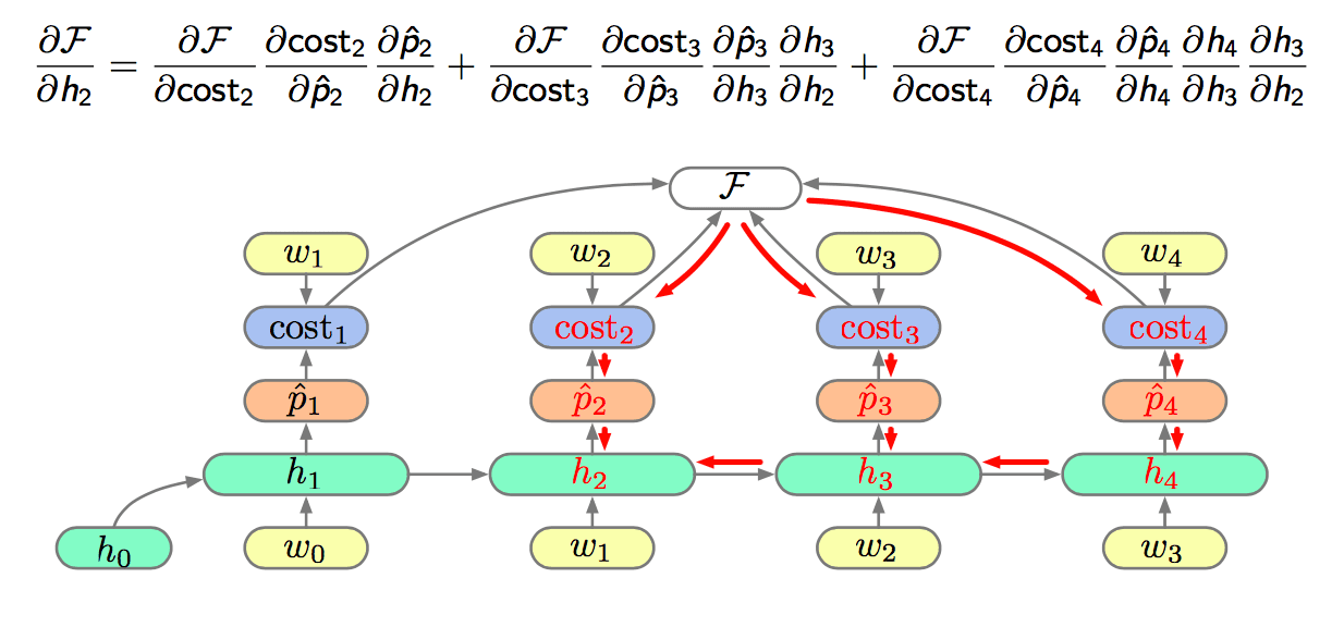
TBPTT
If we break these dependencies after a fixed number of time steps we get Truncated Back Propagation Through Time (TBPTT).
where
\[ h_n = g(V_xx_n + V_hh_{n-1} + c) = g(z_n) \]
\[ \frac{\partial h_n}{\partial z_n} = diag(g'(z_n)) \]
The core of the recurrent product is the repeated multiplication of \(V_h\). If the largest eigenvalue of \(V_h\) is:
- \(1\), then gradient will propagate,
- \(>1\), the product will grow exponentially (explode),
- \(<1\), the prodcut shrinks exponentially (vanishes).
Most of the time the spectral radius of \(V_h\) is small. The result is that the gradient vanishes and long range dependencies are not learnt.
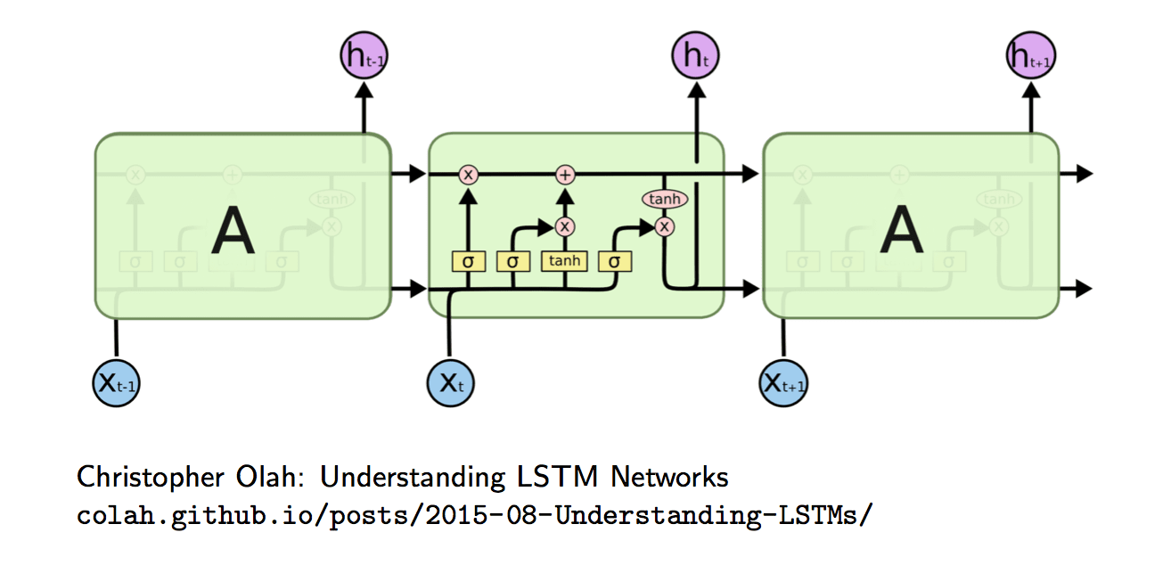
Long Short Term Memory (LSTM)
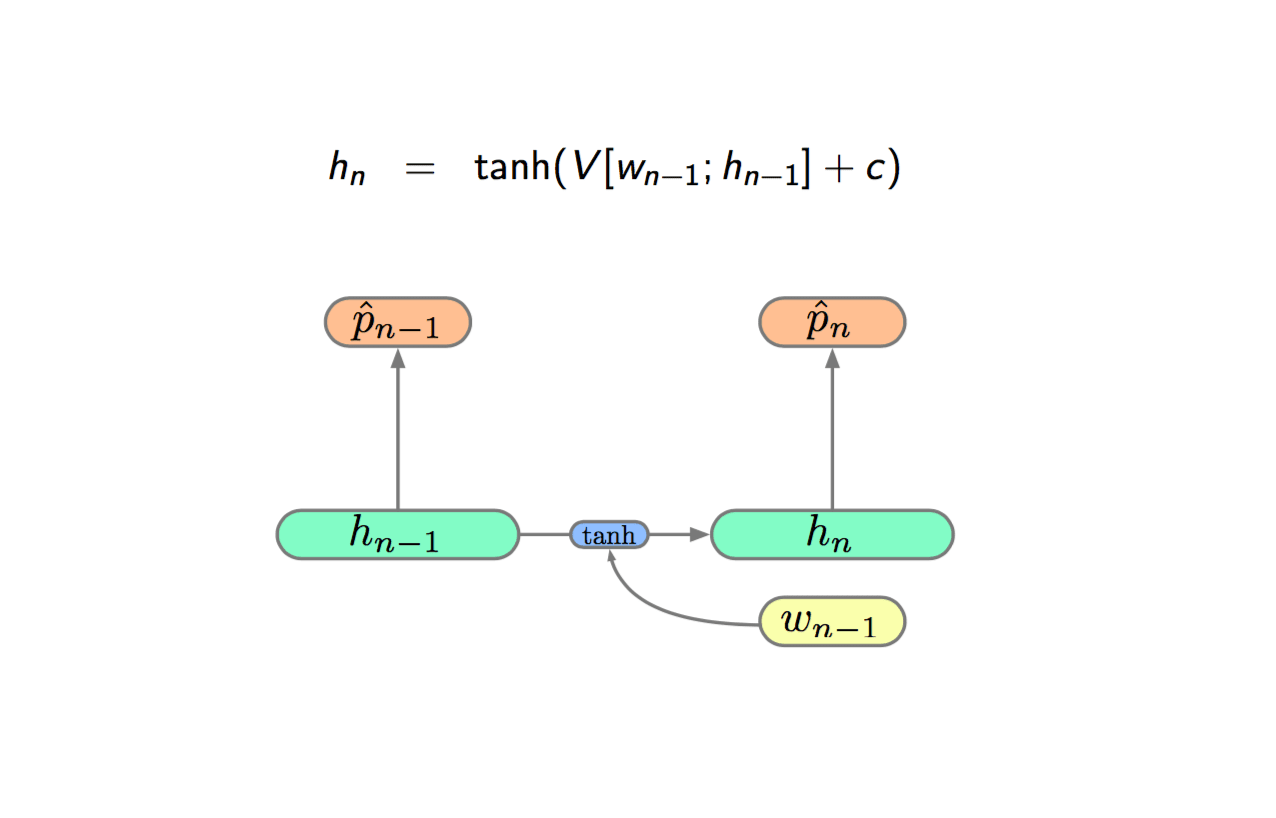
The original RNN is:
Then adding a linear layer of current input and previous state and then going through a tanh non-linearity before passing to the current state:
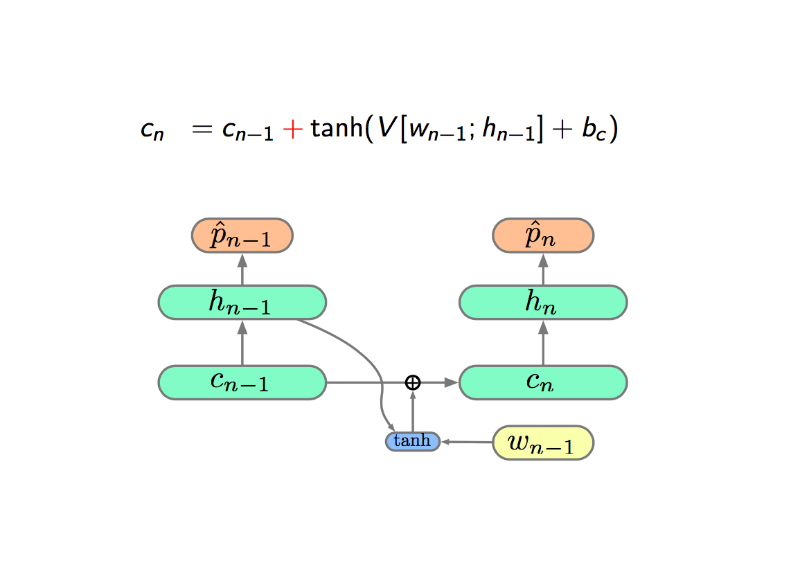
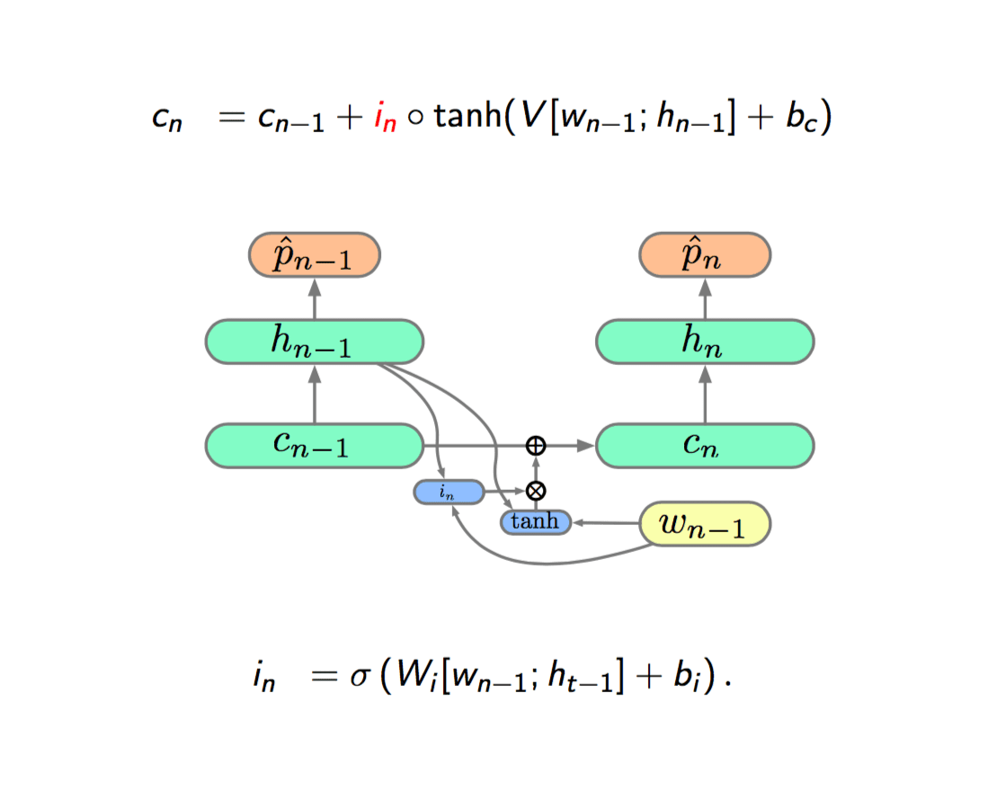
The next step is to introduce an extra hidden layer called cell-state (\(c\)), and think it as our memory. The really cool thing is that propagation is additive. The key innovation of LSTM is replacing the multiplication with sum.
How to balance the grow of addition?
The method is called Gating. So we are going to do is gating the input of the hidden layer, which is called input gate, represented by \(i\). The gate in neural network, is to compute a non-linearity, which is bound between 0 and 1. We think it like a switch, if 1, we turn on the connection and if 0, we shut off the connection. The key thing is the gate is not a decret binary function but a continuous function, thus we can differentiate and back propagation through it.
If the gate is 1, the input would contribute to the current state, if the gate is 0, the input would not affect the current state, so the gate gives state ability to ignore the input.
We already have the ability to include or ignore the input, but we can't forget things. So next we are going to add a forget gate, represented by \(f\).
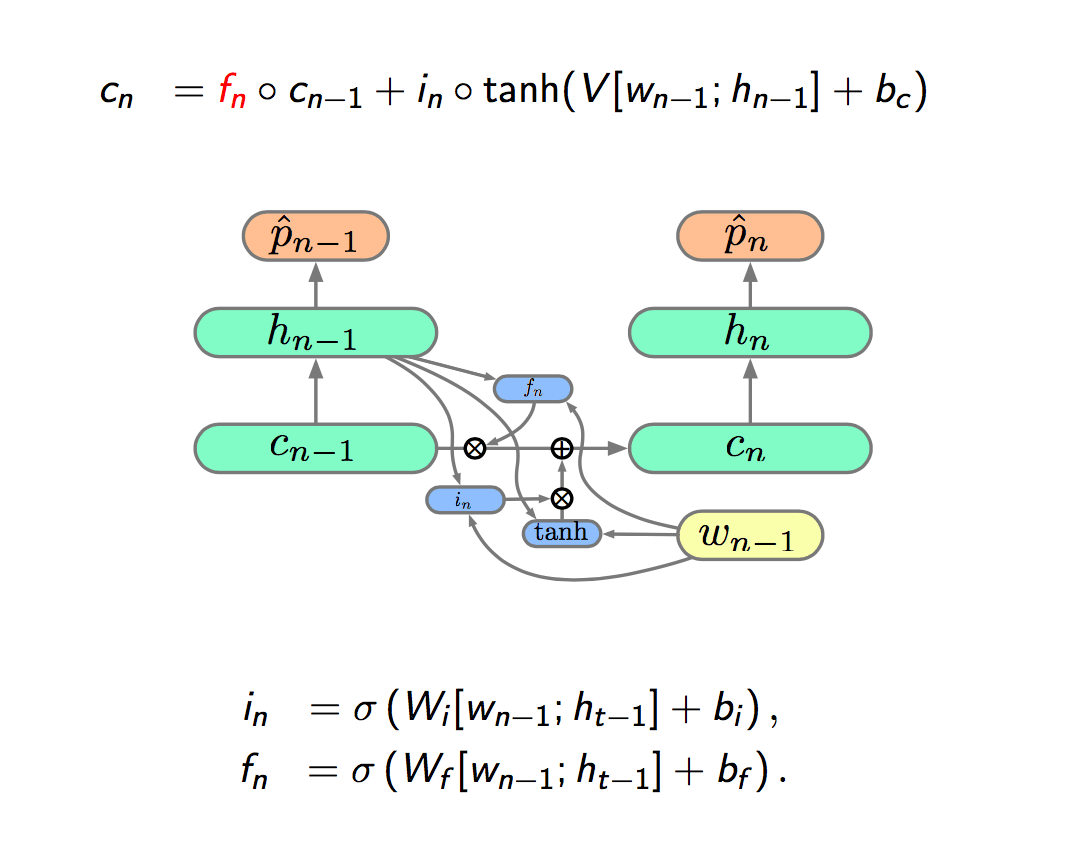
So given the \(i\) and \(f\), our network has the ability to include something new and decide what to remember depend on the input to the next cell state.
The final step is to add a output gate, represented by \(o\), between the cell state to the current state.
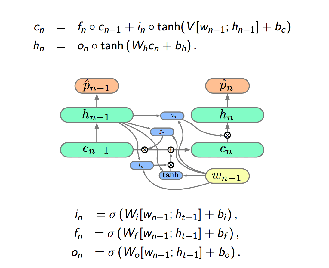
The LSTM cell : \[ c_n = f_n \circ c_{n-1} + i_n \circ \hat{c_n} \]
\[ \begin{align} \hat{c_n} &= \tanh (W_c[w_{n-1};h_{t-1}] + b_c)\\ h_n &= o_n \circ \tanh (W_h c_n + b_h)\\ i_n &= \sigma (W_i[w_{n-1}; h_{t-1}] + b_i)\\ f_n &= \sigma (W_f[w_{n-1}; h_{t-1}] + b_f)\\ o_n &= \sigma (W_o[w_{n-1}; h_{t-1}] + b_o) \end{align} \]
Gated Recurrent Unit (GRU)
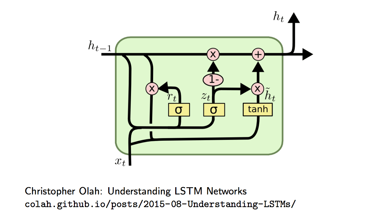
LSTMs and GRUs
Good
- Careful initialisation and optimisation of vanilla RNNs can enable then to learn long(ish) dependencies, but gated additive cells, like the LSTM and GRU, often just work.
- The (re)introduction of LSTMs has been key to many recent developments, e.g. Neural Machine Translation, Speech Recognition, TTS, etc.
Bad
- LSTMs and GRUs have considerably more parameters and computation per memory cell than a vanilla RNN, as such they have less memory capacity per parameter.
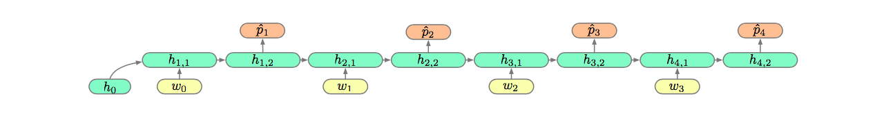
Deep RNN LMs
The memory capacity of an RNN can be increased by employing a larger hidden layer \(h_n\), but a linear increase in \(h_n\) results in quadratic increase in model size and compution:
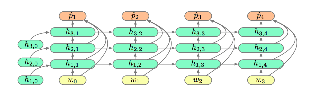
Alternatively we can increase depth in the time dimension. This improves the representational ability, but not the memory capacity.
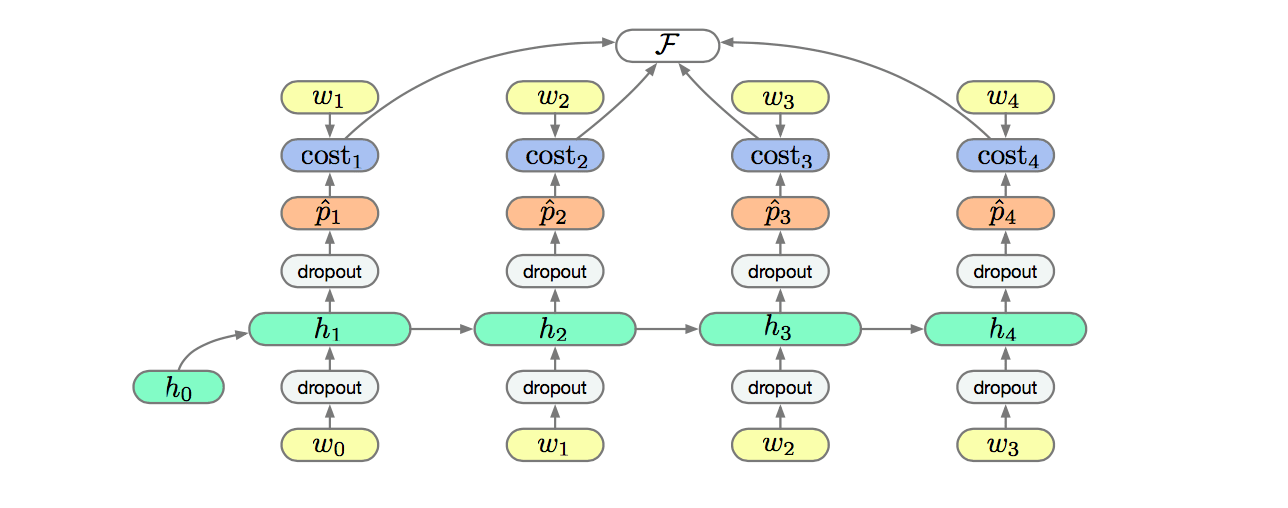
Regularisation : Dropout
Large recurrent networks often overfit their training data by memorising the sequences observed. Such models generalise poorly to novel sequences.
A common approach in Deep Learning is to overparametrise a model, such that it could easily memorise the training data, and then heavily regularise it to facilitate generalisation.
The regularisation method of choice is often Dropout.
Dropout is ineffective when applied to recurrent connections, as repeated random masks zero all hidden units in the limit. The most common solution is to only apply dropout to non-recurrent connections.
Summary
Long Range Dependencies
- The repeated multiplication of the recurrent weights \(V\) lead to vanishing (or exploding) gradients,
- additive gated architectures, such as LSTMs, significantly reduce this issue.
Deep RNNs
- Increasing the size of the recurrent layer increases memory capacity with a quadratic slow down,
- deepening networks in both dimensions can improve their representational efficiency and memory capacity with a linear complexity cost.
Large Vocabularies
- Large vocabularies, \(V > 10^4\), lead to slow softmax calculations,
- reducing the number of vector matrix products evaluated,by factorising the softmax or sampling, reduces the training overhead significantly.
- Different optimisations have different training and evaluation complexities which should be considered.
Readings
Textbook
- Deep Learning, Chapter 10
Blog Posts